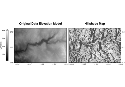
pygmt.grdgradient
- pygmt.grdgradient(grid, *, azimuth=None, direction=None, radiance=None, outgrid=None, normalize=None, tiles=None, region=None, slope_file=None, verbose=None, coltypes=None, interpolation=None, **kwargs)[source]
Compute the directional derivative of the vector gradient of the data.
Can accept
azimuth,direction, andradianceinput to create the resulting gradient.Full option list at https://docs.generic-mapping-tools.org/latest/grdgradient.html
Aliases:
A = azimuth
D = direction
E = radiance
G = outgrid
N = normalize
Q = tiles
R = region
S = slope_file
V = verbose
f = coltypes
n = interpolation
- Parameters
grid (str or xarray.DataArray) – The file name of the input grid or the grid loaded as a DataArray.
outgrid (str or None) – The name of the output netCDF file with extension .nc to store the grid in.
azimuth (int or float or str or list) – azim[/azim2]. Azimuthal direction for a directional derivative; azim is the angle in the x,y plane measured in degrees positive clockwise from north (the +y direction) toward east (the +x direction). The negative of the directional derivative, \(-(\frac{dz}{dx}\sin(\mbox{azim}) + \ \frac{dz}{dy}\cos(\mbox{azim}))\), is found; negation yields positive values when the slope of \(z(x,y)\) is downhill in the azim direction, the correct sense for shading the illumination of an image by a light source above the x,y plane shining from the azim direction. Optionally, supply two azimuths, azim/azim2, in which case the gradients in each of these directions are calculated and the one larger in magnitude is retained; this is useful for illuminating data with two directions of lineated structures, e.g., 0/270 illuminates from the north (top) and west (left). Finally, if azim is a file it must be a grid of the same domain, spacing and registration as grid that will update the azimuth at each output node when computing the directional derivatives.
direction (str) –
[a][c][o][n]. Find the direction of the positive (up-slope) gradient of the data. The following options are supported:
a - Find the aspect (i.e., the down-slope direction)
c - Use the conventional Cartesian angles measured counterclockwise from the positive x (east) direction.
o - Report orientations (0-180) rather than directions (0-360).
n - Add 90 degrees to all angles (e.g., to give local strikes of the surface).
radiance (str or list) – [m|s|p]azim/elev[+aambient][+ddiffuse][+pspecular][+sshine]. Compute Lambertian radiance appropriate to use with pygmt.Figure.grdimage and pygmt.Figure.grdview. The Lambertian Reflection assumes an ideal surface that reflects all the light that strikes it and the surface appears equally bright from all viewing directions. Here, azim and elev are the azimuth and elevation of the light vector. Optionally, supply ambient [0.55], diffuse [0.6], specular [0.4], or shine [10], which are parameters that control the reflectance properties of the surface. Default values are given in the brackets. Use s for a simpler Lambertian algorithm. Note that with this form you only have to provide azimuth and elevation. Alternatively, use p for the Peucker piecewise linear approximation (simpler but faster algorithm; in this case azim and elev are hardwired to 315 and 45 degrees. This means that even if you provide other values they will be ignored.).
[e|t][amp][+aambient][+ssigma][+ooffset]. The actual gradients \(g\) are offset and scaled to produce normalized gradients \(g_n\) with a maximum output magnitude of amp. If amp is not given, default amp = 1. If offset is not given, it is set to the average of \(g\). The following forms are supported:
True - Normalize using \(g_n = \mbox{amp}\ (\frac{g - \mbox{offset}}{max(|g - \mbox{offset}|)})\)
e - Normalize using a cumulative Laplace distribution yielding: \(g_n = \mbox{amp}(1 - \ \exp{(\sqrt{2}\frac{g - \mbox{offset}}{\sigma}))}\), where \(\sigma\) is estimated using the L1 norm of \((g - \mbox{offset})\) if it is not given.
t - Normalize using a cumulative Cauchy distribution yielding: \(g_n = \ \frac{2(\mbox{amp})}{\pi}(\tan^{-1}(\frac{g - \ \mbox{offset}}{\sigma}))\) where \(\sigma\) is estimated using the L2 norm of \((g - \mbox{offset})\) if it is not given.
As a final option, you may add +aambient to add ambient to all nodes after gradient calculations are completed.
tiles (str) – c|r|R. Controls how normalization via
normalizeis carried out. When multiple grids should be normalized the same way (i.e., with the same offset and/or sigma), we must pass these values vianormalize. However, this is inconvenient if we compute these values from a grid. Use c to save the results of offset and sigma to a statistics file; if grid output is not needed for this run then do not specifyoutgrid. For subsequent runs, just use r to read these values. Using R will read then delete the statistics file.region (str or list) – xmin/xmax/ymin/ymax[+r][+uunit]. Specify the region of interest.
slope_file (str) – Name of output grid file with scalar magnitudes of gradient vectors. Requires
directionbut makesoutgridoptional.Select verbosity level [Default is w], which modulates the messages written to stderr. Choose among 7 levels of verbosity:
q - Quiet, not even fatal error messages are produced
e - Error messages only
w - Warnings [Default]
t - Timings (report runtimes for time-intensive algorithms);
i - Informational messages (same as
verbose=True)c - Compatibility warnings
d - Debugging messages
coltypes (str) – [i|o]colinfo. Specify data types of input and/or output columns (time or geographical data). Full documentation is at https://docs.generic-mapping-tools.org/latest/gmt.html#f-full.
interpolation (str) –
[b|c|l|n][+a][+bBC][+c][+tthreshold]. Select interpolation mode for grids. You can select the type of spline used:
b for B-spline
c for bicubic [Default]
l for bilinear
n for nearest-neighbor
- Returns
ret (xarray.DataArray or None) – Return type depends on whether the
outgridparameter is set:xarray.DataArrayifoutgridis not setNone if
outgridis set (grid output will be stored in file set byoutgrid)
